SUBGRADIENT DESCENT

Subgradient descent is an extension of gradient descent for non-smooth convex functions. Unlike classical gradient descent, which requires differentiability, subgradient descent allows optimization over functions that have kinks or discontinuities in their gradients.

The Subgradient Descent Algorithm

Given an initial point:

x_{0} \in R^{n}

and a subgradient:

g \in \partial f (x),

the update rule follows:

x_k + 1 := x_{k} - γ g_{k},

where $g_{k}$ is any subgradient of $f (x)$ at $x_{k}$ .

Important Note:

Negative subgradients are not necessarily descent directions.

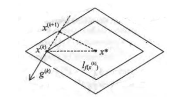
Subgradient Descent Does Not Descend.png

Negative subgradients are not necessarily descent directions.png

This differs from classical gradient descent, where the negative gradient always points towards decreasing function values.

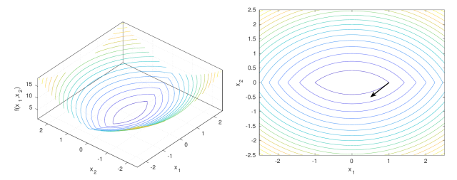
Example of Subgradient Descent

Consider the function:

f (x) = | x_{1} - x_{2} | + 0.2 | x_{1} + x_{2} |

with a subgradient at $(1, 1)$ :

g (1, 1) = (1.2, - 0.8)

Since $f (x)$ is not smooth, any subgradient could be used at each step, leading to different update directions.

An important property:

f (x_k + 1) \geq f (x_{k})

shows that subgradient descent does not necessarily decrease function values at each step.

Additionally:

\|x\_{k+1} - x^_\| \leq \|x_k - x^_\|

suggests that the iterates remain bounded, even if the function value does not strictly decrease.

How to Choose a Step Size?

In subgradient descent, the step size $γ_{k}$ plays a crucial role. There are several common choices:

1. Diminishing Step Size:

A common approach is to use a sequence $γ_{k}$ that tends to zero:

x_k + 1 = x_{k} - γ_{k} \frac{\partial^{+} f (x_{k})}{∥ \partial^{+} f (x_{k}) ∥},

Remark:

The plus sign ( $+$ ) in $\partial^{+} f (x_{k})$ indicates that we are selecting a particular subgradient from the subdifferential set $\partial f (x)$ . There are several possible interpretations:

Selecting the steepest subgradient
- If multiple subgradients exist (e.g., at a nondifferentiable point), we might choose the one with the largest norm or the steepest > descent direction.
- This is useful in algorithms like normalized subgradient descent to ensure consistent step sizes.
Selecting a specific element in a structured way
- Some optimization methods require a deterministic or structured choice of subgradient.
- The plus sign may indicate a particular rule for selecting a subgradient, e.g., the right-hand derivative in one-dimensional cases.
Right subgradient in nonsmooth analysis
- In some contexts (like directional derivatives), $\partial^{+} f (x)$ may refer to the right subdifferential, meaning we consider > subgradients corresponding to increasing values of $x$ .

where $γ_{k}$ satisfies:

γ * k \to 0, \sum * {k = 0}^{\infty} γ_{k} = \infty .

Three typical choices:

$γ_{k} = \frac{c}{k}$ , where $c$ is a constant.
$γ_{k} = \frac{x_{0}}{k^{ρ}}, 0 < ρ \leq 1$ .
$γ_{k} = \frac{γ_{0}}{k ∥ g_{k} ∥}$ .

2. If the optimal function value $f (x^{*})$ is known:

The update rule can be modified as:

x_k + 1 = x^{k} - \frac{\partial^{+} f (x^{k})}{∥ \partial^{+} f (x^{k}) ∥^{2}} f (x^{k}) - f (x^{\*})

3. Using the best observed function value:

Define:

f * k^{best} = min * 1 \leq i \leq k f (x_{i}),

and use:

f^{\*} = min_{k} f (x_{k}) .

This ensures convergence by tracking the best function value observed so far.

Convergence of Subgradient Descent

Lipschitz Convex Functions

If $f : R^{n} \to R$ is convex and B-Lipschitz continuous with a global minimum $x^{*}$ , and:

∥ x_{0} - x^{\*} ∥ \leq R,

then choosing the constant step size:

γ := \frac{R}{B \sqrt{T}}

yields:

\frac{1}{T} \sum_{t = 0}^{T - 1} f (x_{t}) - f (x^{\*}) \leq \frac{R B}{\sqrt{T}} .

Strongly Convex Functions

If $f : R^{n} \to R$ is strongly convex with parameter $μ > 0$ , then using the decreasing step size:

γ_{k} = \frac{2}{μ (k + 1)}, t > 0,

yields:

f (\frac{2}{K (K + 1)} \sum_{i = 1}^{K} i x_{i}) - f (x^{\*}) \leq \frac{2 B^{2}}{μ (K + 1)} .

where:

B = max_{k} ∥ g_{k} ∥ .

This shows that subgradient descent converges slower than standard gradient descent, but still guarantees progress over time.